Supply & Pricing

Professor/Lecturer Ellmann's Course Materials Page

Supply & Pricing

Short‐Run Supply

In determining how much output to supply, the firm's objective is to maximize profits subject to two constraints: the consumers' demand for the firm's product and the firm's costs of production. Consumer demand determines the price at which a perfectly competitive firm may sell its output. The costs of production are determined by the technology the firm uses. The firm's profits are the difference between its total revenues and total costs.

Total revenue and marginal revenue. A firm's total revenue is the dollar amount that the firm earns from sales of its output. If a firm decides to supply the amount Q of output and the price in the perfectly competitive market is P, the firm's total revenue is

A firm's marginal revenue is the dollar amount by which its total revenue changes in response to a 1-unit change in the firm's output. If a firm in a perfectly competitive market increases its output by 1 unit, it increases its total revenue by P × 1 = P. Hence, in a perfectly competitive market, the firm's marginal revenue is just equal to the market price, P.

Short-run profit maximization. A firm maximizes its profits by choosing to supply the level of output where its marginal revenue equals its marginal cost. When marginal revenue exceeds marginal cost, the firm can earn greater profits by increasing its output. When marginal revenue is below marginal cost, the firm is losing money, and consequently, it must reduce its output. Profits are therefore maximized when the firm chooses the level of output where its marginal revenue equals its marginal cost.

To illustrate the concept of profit maximization, consider again the example of the firm that produces a single good using only two inputs, labor and capital. In the short-run, the amount of capital the firm uses is fixed at 1 unit. Assume that this firm is competing with many other firms in a perfectly competitive market. The price of the good sold in this market is $10 per unit. The firm's costs of production for different levels of output are the same as those considered in the numerical examples of the previous section, Theory of the Firm. These costs, along with the firm's total and marginal revenues and its profits for different levels of output, are reported in Table 1 .

TABLE 1

Firm Output, Revenues, Costs, and Profits

Total product	Total revenue	Marginal revenue	Total cost	Average total cost	Marginal cost	Firm profits
0	$0	—	$100	—	—	−$100
5	50	$10	120	$24.00	$4.0	−70
15	150	10	140	9.33	2.0	10
23	230	10	160	6.96	2.5	70
27	270	10	180	6.66	5.0	90
29	290	10	200	6.90	10.0	90
30	300	10	220	7.33	20.0	80

Because the price of the good is $10, the firm's total revenue is 10 × total product. The firm's marginal revenue is equal to the price of $10 per unit of total product. Notice that the marginal cost of the 29th unit produced is $10, while the marginal revenue from the 29th unit is also $10. Hence, the firm maximizes its profits by choosing to produce exactly 29 units of output. In choosing to produce 29 units of output, the firm earns $90 ($290 − 200) in profits.

Graphical illustration of short-run profit maximization. The marginal revenue, marginal cost, and average total cost figures reported in the numerical example of Table 1 are shown in the graph in Figure 1 .

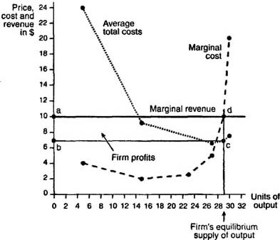
Figure 1

The firm's short-run, profit-maximizing decision

The firm's equilibrium supply of 29 units of output is determined by the intersection of the marginal cost and marginal revenue curves (point d in Figure 1 ). When the firm produces 29 units of output, its average total cost is found to be $6.90 (point con the average total cost curve in Figure 1 ). The firm's profits are therefore given by the area of the shaded rectangle labeled abed.

The area of this rectangle is easily calculated. The length of the rectangle is 29. The width is the difference between the market price (the firm's marginal revenue), $10, and the firm's average cost of producing 29 units, $6.90. This difference is ($10 × $6.90) = $3.10. Hence, the area of rectangle abed is 29 × $3.1 = $90, the same amount reported in Table 1 . In general, the firm makes positive profits whenever its average total cost curve lies below its marginal revenue curve.

Short-run losses and the shut-down decision. When the firm's average total cost curve lies above its marginal revenue curve at the profit maximizing level of output, the firm is experiencing losses and will have to consider whether to shut down its operations. In making this determination, the firm will take into account its average variable costs rather than its average total costs. The difference between the firm's average total costs and its average variable costs is its average fixed costs.The firm must pay its fixed costs (for example, its purchases of factory space and equipment), regardless of whether it produces any output. Hence, the firm's fixed costs are considered sunk costs and will not have any bearing on whether the firm decides to shut down. Thus, the firm will focus on its average variable costs in determining whether to shut down.

If the firm's average variable costs are less than its marginal revenue at the profit maximizing level of output, the firm will not shut down in the short-run. The firm is better off continuing its operations because it can cover its variable costs and use any remaining revenues to pay off some of its fixed costs. The fact that the firm can pay its variable costs is all that matters because in the short-run, the firm's fixed costs are sunk; the firm must pay its fixed costs regardless of whether or not it decides to shut down. Of course, the firm will not continue to incur losses indefinitely. 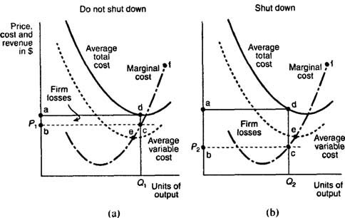In the long-run, a firm that is incurring losses will have to either shut down or reduce its fixed costs by changing its fixed factors of production in a manner that makes the firm's operations profitable.

The case where the firm is incurring short-run losses but continues to operate is illustrated graphically in Figure 2 (a). At the market price, P₁, the firm's profit maximizing quantity is Q₁. At this quantity, the firm's average total cost curve lies above its marginal revenue curve, which is the flat, dashed line denoting the price level, P₁. The firm's average variable cost curve, however, lies below its marginal revenue curve, implying that the firm is able to cover its variable costs. The firm's losses from producing quantity Q₁ at price P₁ are given by the area of the shaded rectangle, abcd. Despite these losses, the firm will decide not to shut down in the short-run because it receives enough revenue to pay for its variable costs.

Figure 2

The firm's short-run shut-down decision

Figure 2 (b) depicts a different scenario in which the firm's average total cost and average variable cost curves both lie above its marginal revenue curve, which is the dashed line at price P₂. The firm's losses are given by the area of the shaded rectangle, abed. In this situation, the firm will have to shut down in the short-run because it is unable to cover even its variable costs. As a general rule, a firm will shut down production whenever its average variable costs exceed its marginal revenue at the profit maximizing level of output. If this is not the case, the firm may continue its operations in the short-run, even though it may be experiencing losses.

Short-run supply curve. The firm's short-run supply curve is the portion of its marginal cost curve that lies above its average variable cost curve. As the market price rises, the firm will supply more of its product, in accordance with the law of supply. If, however, the market price, which is the firm's marginal revenue curve, falls below the firm's average variable cost, the firm will shut down and supply zero output.

The firm's short-run supply curve is illustrated in Figures 2 (a) and 2 (b). Here, the firm's short-run supply curve is the portion of the marginal cost curve labeled ef. The market short-run supply curve, like the market demand curve, is simply the horizontal summation of all the individual firms' short-run supply curves.

Long‐Run Supply

In the long-run, firms can vary all of their input factors. The ability to vary the amount of input factors in the long-run allows for the possibility that new firms will enter the market and that some existing firms will exit the market. Recall that in a perfectly competitive market, there are no barriers to the entry and exit of firms. New firms will be tempted to enter the market if some of the existing firms in the market are earningpositive economic profits. Alternatively, existing firms may choose to leave the market if they are earning losses. For these reasons, the number of firms in a perfectly competitive market is unlikely to remain unchanged in the long-run.

Zero economic profits. The entry and exit of firms, which is possible in the long-run, will eventually cause each firm's economic profits to fall to zero. Hence, in the long-run each firm earns normal profits. If some firms are earning positive economic profits in the short-run, in the long-run new firms will enter the market and the increased competition will reduce all firms' economic profits to zero. Firms that are earning negative economic profits (losses) in the short-run will have to either make some changes in their fixed factors of production in the long-run or choose to leave the market in the long-run. A perfectly competitive market achieves long-run equilibrium when all firms are earning zero economic profits and when the number of firms in the market is not changing.

Minimization of long-run average total cost. In the long-run, a perfectly competitive firm can adjust the amount it uses of all factor inputs, including those that are fixed in the short-run. For example, in the long-run, the firm can adjust the size of its factory. In making these adjustments, the firm will seek to minimize its long-run average total cost. If, in the short-run, the firm is operating below its minimum efficient scale and experiencing economies of scale, in the long-run it can adjust its use of factor inputs so as to increase its output to the minimum efficient scale level.

Alternatively, if the firm is experiencing diseconomies of scale because its short-run level of output exceeds its minimum efficient scale, in the long-run the firm can adjust its use of factor inputs so as to reduce its output to the minimum efficient scale level. Thus, in the long-run the firm will be operating at the minimum point of its long-run average total cost curve.

Graphical illustration of long-run profit maximization. The long-run equilibrium for an individual firm in a perfectly competitive market is illustrated in Figure 1 .

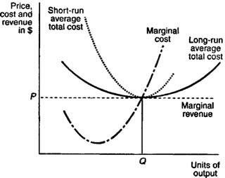
Figure 1

The firm's long-run profit-maximizing decision

The profit maximizing level of output, where marginal cost equals marginal revenue, results in an equilibrium quantity of Q units of output. Because the firm's average total costs per unit equal the firm's marginal revenue per unit, the firm is earning zero economic profits. Furthermore, the firm is shown to be producing at the minimum point of its long-run average total cost curve, at the minimum efficient scale level of output.

Long-run market supply curve. The short-run market supply curve is just the horizontal summation of all the individual firm's supply curves. The long-run market supply curve is found by examining the responsiveness of short-run market supply to a change in market demand. Consider the market demand and supply curves depicted in Figures 2 (a) and 2 (b). Here, the market demand curves are labeled D₁, and D₂, while the short-run market supply curves are labeled S₁ and S₂.

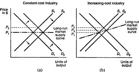
Figure 2

Long-run market supply curves

Figure 2 (a) depicts demand and supply curves for a market or industry in which firms face constant costs of production as output increases. At the intersection of D₁ and S₁, the market is in long-run equilibrium at a market price of P₁. An increase in demand from D₁ to D₂ results in a new, higher market price of P₂. In the short-run, existing firms in this market will earn positive economic profits. In the long-run, however, new firms will enter, causing short-run market supply to shift from S₁ to S₂and driving the market price back down to P₁. The long-run market supply curve is therefore given by the horizontal line at the market price, P₁

Figure 2 (b) depicts demand and supply curves for a market or industry in which firms face increasing costs of production as output increases. Starting from a market price of P₁, an increase in demand from D₁ to D₂ increases the market price to P₂. In the short-run, firms are earning positive economic profits. In the long-run, new firms will enter the market, the short-run supply curve will shift from S₁ to S₂, and the new market price will be P₃. The new, long-run market price of P₃ is greater than the old market price of P₁ because in an increasing-cost industry, the firm's average total costs rise as it produces more output. Thus, the long-run market supply curve in an increasing-cost industry will be positively sloped.

Enter supporting content here